The Mathematics of “Filling the Triangle”

I’ve been fascinated by the triangle offense for a long time. I think it is a beautiful way to play basketball, and the right way to play basketball, in the half-court, a “system-based” way to play. For those of you that are interested, I highly recommend Tex Winter’s classic book on the topic.

There is this brief video as well where Tex Winter explains how the triangle offense and a basketball are grounded in geometric principles:

 

I don’t think people recognize though how deep of a geometry problem this is actually. Looking at when the triangle is filled, as in the video above, we have the following situation:

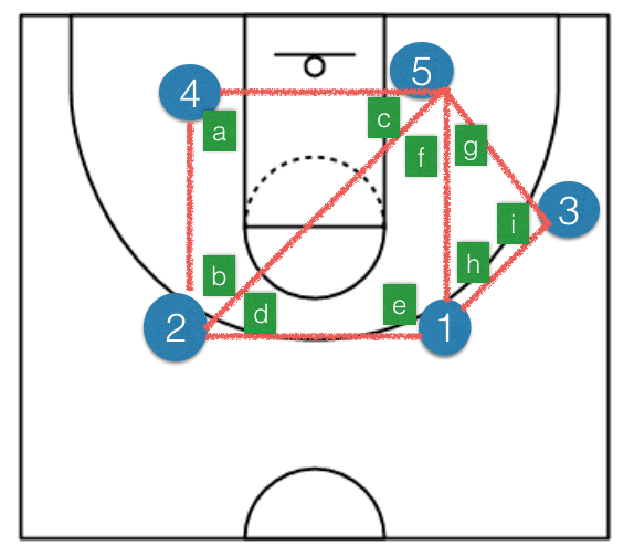
The problem I wanted to study was given 5 players’ random positions on the court, could a series of equations be solved yielding (x,y) coordinates that would yield where players should “go” to fill the triangle? 

Using simple geometry, from the diagram above, we see that each player’s position in the triangle offense is governed by the following system of nonlinear equations:

Further, the angles obviously must satisfy the following constraints:

Finally, we require that each player be about 15-20 feet apart in the triangle offense (because the offense is predicated on spacing), and thus have some additional constraints:

Solving this highly nonlinear system of equations with constraints is not a trivial problem! It fact, because of the high degree of nonlinearity and dimension of the problem, it is safe to assume that no closed-form solution exists, and therefore, must be solved numerically.

For this task, we used MATLAB, and experimented with the lsqnonlin() and fsolve() commands. The only issue is that (as with all such numerical algorithms) convergence depends very highly on the choice of initial conditions. It is very difficult to choose a priori this many initial conditions, so I wrote a script that randomized initial conditions. I then ran several numerical experiments and obtained the following results:

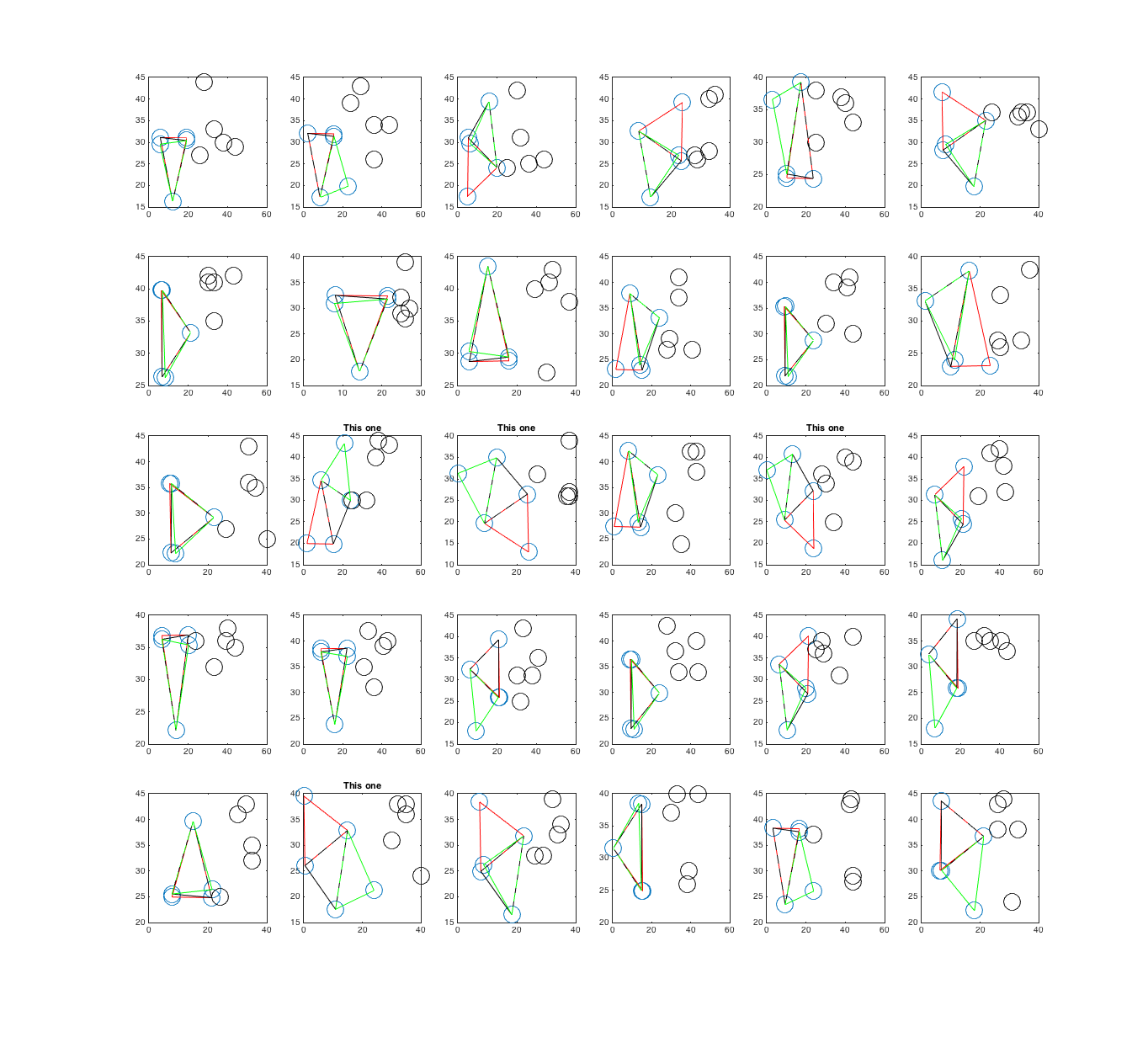
In the plot above, I have labeled the plots that converged to the triangle formation with the title “this one”. In addition, the five black circles denote the initial positions of the players on the court before they fill the triangles in the offense. One sees just by the diagram above, how difficult such a problem is to solve mathematically, even through a numerical approach. Running more trials would perhaps yield better results, but, it works! I am truly fascinated by this. In the coming days, I will work on optimizing the numerical algorithm, and post my updates as they come.

Here is an animation of one of the scenarios above when the algorithm converges correctly:

In this animation above, the black dots represent the positions of the players on the court. They begin at initial (random) positions and attempt to fill the triangles as described above.

Thanks for reading!