An interesting machine learning problem: Can one figure out the relationship between the popular vote margin, voter turnout, and the percentage of electoral college votes a candidate wins? Going back to the election of John Quincy Adams, the raw data looks like this:
| Electoral College | Party | Popular vote Margin (%) |
Percentage of EC |
|
| John Quincy Adams | D.-R. | -0.1044 | 0.27 | 0.3218 |
| Andrew Jackson | Dem. | 0.1225 | 0.58 | 0.68 |
| Andrew Jackson | Dem. | 0.1781 | 0.55 | 0.7657 |
| Martin Van Buren | Dem. | 0.14 | 0.58 | 0.5782 |
| William Henry Harrison | Whig | 0.0605 | 0.80 | 0.7959 |
| James Polk | Dem. | 0.0145 | 0.79 | 0.6182 |
| Zachary Taylor | Whig | 0.0479 | 0.73 | 0.5621 |
| Franklin Pierce | Dem. | 0.0695 | 0.70 | 0.8581 |
| James Buchanan | Dem. | 0.12 | 0.79 | 0.5878 |
| Abraham Lincoln | Rep. | 0.1013 | 0.81 | 0.5941 |
| Abraham Lincoln | Rep. | 0.1008 | 0.74 | 0.9099 |
| Ulysses Grant | Rep. | 0.0532 | 0.78 | 0.7279 |
| Ulysses Grant | Rep. | 0.12 | 0.71 | 0.8195 |
| Rutherford Hayes | Rep. | -0.03 | 0.82 | 0.5014 |
| James Garfield | Rep. | 0.0009 | 0.79 | 0.5799 |
| Grover Cleveland | Dem. | 0.0057 | 0.78 | 0.5461 |
| Benjamin Harrison | Rep. | -0.0083 | 0.79 | 0.58 |
| Grover Cleveland | Dem. | 0.0301 | 0.75 | 0.6239 |
| William McKinley | Rep. | 0.0431 | 0.79 | 0.6063 |
| William McKinley | Rep. | 0.0612 | 0.73 | 0.6532 |
| Theodore Roosevelt | Rep. | 0.1883 | 0.65 | 0.7059 |
| William Taft | Rep. | 0.0853 | 0.65 | 0.6646 |
| Woodrow Wilson | Dem. | 0.1444 | 0.59 | 0.8192 |
| Woodrow Wilson | Dem. | 0.0312 | 0.62 | 0.5217 |
| Warren Harding | Rep. | 0.2617 | 0.49 | 0.7608 |
| Calvin Coolidge | Rep. | 0.2522 | 0.49 | 0.7194 |
| Herbert Hoover | Rep. | 0.1741 | 0.57 | 0.8362 |
| Franklin Roosevelt | Dem. | 0.1776 | 0.57 | 0.8889 |
| Franklin Roosevelt | Dem. | 0.2426 | 0.61 | 0.9849 |
| Franklin Roosevelt | Dem. | 0.0996 | 0.63 | 0.8456 |
| Franklin Roosevelt | Dem. | 0.08 | 0.56 | 0.8136 |
| Harry Truman | Dem. | 0.0448 | 0.53 | 0.5706 |
| Dwight Eisenhower | Rep. | 0.1085 | 0.63 | 0.8324 |
| Dwight Eisenhower | Rep. | 0.15 | 0.61 | 0.8606 |
| John Kennedy | Dem. | 0.0017 | 0.6277 | 0.5642 |
| Lyndon Johnson | Dem. | 0.2258 | 0.6192 | 0.9033 |
| Richard Nixon | Rep. | 0.01 | 0.6084 | 0.5595 |
| Richard Nixon | Rep. | 0.2315 | 0.5521 | 0.9665 |
| Jimmy Carter | Dem. | 0.0206 | 0.5355 | 0.55 |
| Ronald Reagan | Rep. | 0.0974 | 0.5256 | 0.9089 |
| Ronald Reagan | Rep. | 0.1821 | 0.5311 | 0.9758 |
| George H. W. Bush | Rep. | 0.0772 | 0.5015 | 0.7918 |
| Bill Clinton | Dem. | 0.0556 | 0.5523 | 0.6877 |
| Bill Clinton | Dem. | 0.0851 | 0.4908 | 0.7045 |
| George W. Bush | Rep. | -0.0051 | 0.51 | 0.5037 |
| George W. Bush | Rep. | 0.0246 | 0.5527 | 0.5316 |
| Barack Obama | Dem. | 0.0727 | 0.5823 | 0.6784 |
| Barack Obama | Dem. | 0.0386 | 0.5487 | 0.6171 |
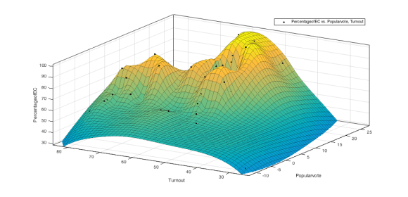
Clearly, the percentage of electoral college votes a candidate depends nonlinearly on the voter turnout percentage and popular vote margin (%) as this non-parametric regression shows:
We therefore chose to perform a nonlinear regression using neural networks, for which our structure was:

As is turns out, this simple neural network structure with one hidden layer gave the lowest test error, which was 0.002496419 in this case.
Now, looking at the most recent national polls for the upcoming election, we see that Hillary Clinton has a 6.1% lead in the popular vote. Our neural network model then predicts the following:
| Simulation | Popular Vote Margin | Percentage of Voter Turnout | Predicted Percentage of Electoral College Votes (+/- 0.04996417) |
| 1 | 0.061 | 0.30 | 0.6607371 |
| 2 | 0.061 | 0.35 | 0.6647464 |
| 3 | 0.061 | 0.40 | 0.6687115 |
| 4 | 0.061 | 0.45 | 0.6726314 |
| 5 | 0.061 | 0.50 | 0.6765048 |
| 6 | 0.061 | 0.55 | 0.6803307 |
| 7 | 0.061 | 0.60 | 0.6841083 |
| 8 | 0.061 | 0.65 | 0.6878366 |
| 9 | 0.061 | 0.70 | 0.6915149 |
| 10 | 0.061 | 0.75 | 0.6951424 |
One sees that even for an extremely low voter turnout (30%), at this point Hillary Clinton can expect to win the Electoral College by a margin of 61.078% to 71.07013%, or 328 to 382 electoral college votes. Therefore, what seems like a relatively small lead in the popular vote (6.1%) translates according to this neural network model into a large margin of victory in the electoral college.
One can see that the predicted percentage of electoral college votes really depends on popular vote margin and voter turnout. For example, if we reduce the popular vote margin to 1%, the results are less promising for the leading candidate:
| Pop.Vote Margin | Voter Turnout % | E.C. % Win | E.C% Win Best Case | E.C.% Win Worst Case |
| 0.01 | 0.30 | 0.5182854 | 0.4675000 | 0.5690708 |
| 0.01 | 0.35 | 0.5244157 | 0.4736303 | 0.5752011 |
| 0.01 | 0.40 | 0.5305820 | 0.4797967 | 0.5813674 |
| 0.01 | 0.45 | 0.5367790 | 0.4859937 | 0.5875644 |
| 0.01 | 0.50 | 0.5430013 | 0.4922160 | 0.5937867 |
| 0.01 | 0.55 | 0.5492434 | 0.4984580 | 0.6000287 |
| 0.01 | 0.60 | 0.5554995 | 0.5047141 | 0.6062849 |
| 0.01 | 0.65 | 0.5617642 | 0.5109788 | 0.6125496 |
| 0.01 | 0.70 | 0.5680317 | 0.5172463 | 0.6188171 |
| 0.01 | 0.75 | 0.5742963 | 0.5235109 | 0.6250817 |
One sees that if the popular vote margin is just 1% for the leading candidate, that candidate is not in the clear unless the popular vote exceeds 60%.

2 replies on “The Relationship Between The Electoral College and Popular Vote”
[…] are my predictions. In a previous post, I described using a neural network algorithm how one could use the current national poll / popular […]